
File:Mandelbrot Components.svg
| |
This is a file from the Wikimedia Commons. Information from its description page there is shown below.
Commons is a freely licensed media file repository. You can help. |
Contents
|
Summary
| Description | |
| Date | 4 March 2009 |
| Source | maxima code from File:Components1.jpg |
| Author | Gringer ( talk) |
Description with Maxima code
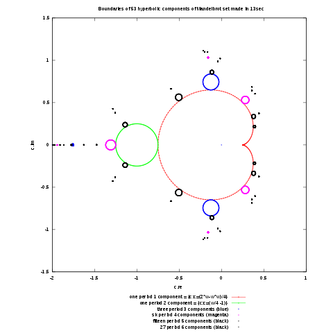
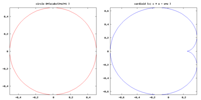
Boundaries of hyperbolic components of Mandelbrot sets are closed curves : cardioids or circles.
Douady-Hubbard-Sullivan theorem (DHS) states that unit circle can be mapped to boundary of hyperbolic component. This relation is defined by boundary equations. Here these equations are used to draw boundaries of hyperbolic components.
Douady-Hubbard-Sullivan theorem
The Douady-Hubbard-Sullivan theorem (DHS) states that the multiplier map  of an attracting periodic orbit is a conformal isomorphism from a hyperbolic component
  of the Mandelbrot set onto the unit disk
  and it extends homeomorpically to the boundaries.
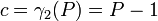
Here it is important that it maps the boundary of a hyperbolic component to the boundary of the unit disk ( = unit circle ) :
and its inverse function maps the unit circle to the boundary of hyperbolic components :
The algorithm
Draft algorithm
The algorithm consist of
- complex mapping circle points to boundary points of a hyperbolic component
Detailed algorithm
For given period  do steps :
- Decide how many points of closed curve you want to draw ( iMax ).
- Compute

- start with

- while
 repeat :
 - compute point of the unit circle in the standard plane
 where
where  is an internal angle,
 - map points onto the parameter plane (complex mapping ) using one of 2 methods :
- using explicit function
 ( it is possible only for periods 1-3)
 - solving implicit equation
 with respect to
  ( it is posible for periods 1-8 using numerical methods)
- using explicit function
- compute new angle

- compute point of the unit circle in the standard plane
Relations between hyperbolic components and unit circle
Definitions
Complex quadratic map :
f(z,c):=z*z+c;
Iterated function (map) :
F(n, z, c) :=
   if n=1 then f(z,c)
   else f(F(n-1, z, c),c);
Multiplier of periodic orbit :
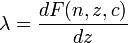
_lambda(n):=diff(F(n,z,c),z,1);
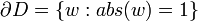
Unit circle  = boundary of unit disk
where coordinates of  point of unit circle in exponential form are :

Boundary equations
Boundary equation
- defines relations between hyperbolic components and unit circle for given period ,
- allows computation of exact coordinates of hyperbolic componenets.
 is boundary polynomial ( implicit function of 2 variables ).
Equations are in papers of Brown,John Stephenson, Wolf Jung. Methods of finding boundary equations are also described in WikiBooks.
For boundary points :

so boundary equations can be in 4 equivalent forms :
| period |
 |
 |
exponential  |
trigonometric |
|---|---|---|---|---|
| 1 | 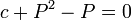 |
 |
 |
 |
| 2 | 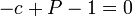 |
 |
 |
 |
For higher periods only P-form is used, because it is the shortest and usefull for computations.
for period 3 :

for period 4 :

for period 5 :

Solving boundary equations with respect to c
Boundary equations for periods:
- 1-3 it can be solved with symbolical methods and give explicit solution :
- >3 it can't be solved explicitly and must be solved numerically with respect to .
period 1
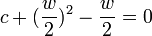
There is only one period 1 component. Because boundary equation is simple :
so it is easy to get inverse multiplier map :
For each internal angle one computes :
- point on unit circle
 ,
, 
- point

Result is a list of boundary points .
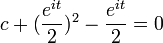
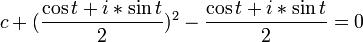
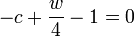
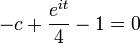
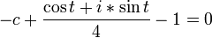
period 2
Because boundary equation is simple :
so it is easy to get inverse multiplier map :
For each internal angle one computes :
- point on unit circle ,

- point

Result is a list of boundary points .
period 3
There are 3 period 3 components Here solution of boundary equation gives 3 inverse multiplier maps  .
.
It is possible in 3 ways :
- Munafo method (every functions maps one half of one component and one half of other component)
- Giarrusso-Fisher method ( one function for one component )
I use functions by Robert Munafo.
(%i3) b3:c^3+2*c^2+(1-P)*c+(P-1)^2=0$
(%i4) solve(b3,c);
(%o4) [
c=(-(sqrt(3)*%i)/2-1/2)*(((P-1)*sqrt(27*P^2-22*P+23))/(6*sqrt(3))-(27*P^2-36*P+25)/54)^(1/3)+
(((sqrt(3)*%i)/2-1/2)*(3*P+1))/(9*(((P-  1)*sqrt(27*P^2-22*P+23))/(6*sqrt(3))-(27*P^2-36*P+25)/54)^(1/3))-2/3,
c=((sqrt(3)*%i)/2-1/2)*
(((P-1)*sqrt(27*P^2-22*P+23))/(6*sqrt(3))-(27*P^2-36*P+25)/54)^(1/3)+
((-(sqrt(3)*%i)/2-1/2)*(3*P+1))/(9*(((P-1)*sqrt(27*P^2-22*P+23)) /(6*sqrt(3))-
(27*P^2-36*P+25)/54)^(1/3))-2/3,
c=(((P-1)*sqrt(27*P^2-22*P+23))/(6*sqrt(3))-(27*P^2-36*P+25)/54)^(1/3)+
(3*P+1)/(9*(((P-1)*sqrt(27*P^2-22*P+23))/(6*sqrt(3))-(27*P^2-36*P+25)/54)^(1/3))
For each internal angle one computes :
- point on unit circle ,

- points :


Result is a list of boundary points .
period 4
Boundary equation  one can find in Mu-Ency. It can't be solved symbolicaly so it must be evaluated numerically.
It is 1 equation with 2 variables. To solve it one has to compute  and put in . Now it is equation with 1 variable and it can be solved numerically.
For each internal angle one computes :
- point on unit circle ,

- Boundary polynomial

- solve boundary equation with respect to . Result is 6 roots ( each for one of 6 period 4 components).
Result is a list of boundary points .
b4(w):=c^6 + 3*c^5 + (w/16+3)* c^4 + (w/16+3)* c^3  - (w/16+2)* (w/16-1)* c^2 - (w/16-1)^3;
l(t):=%e^(%i*t*2*%pi);
iMax:200; /* number of point */
dt:1/iMax;
/* point to point method of drawing */
t:0; /* angle in turns */
w:rectform(ev(l(t), numer)); /* "exponential form prevents allroots from working", code by Robert P. Munafo */
/* compute equation for given w */
per4:expand(b4(w));
/* compute 6 complex roots and save them to the list cc4 */
cc4:allroots(per4);
/*  create new lists and save coordinates  to draw it later */
xx4:makelist (realpart(rhs(cc4[1])), i, 1, 1);
yy4:makelist (imagpart(rhs(cc4[1])), i, 1, 1);
for j:2 thru 6 step 1 do
 block
 (
  xx4:cons(realpart(rhs(cc4[j])),xx4),
  yy4:cons(imagpart(rhs(cc4[j])),yy4)
 );
for i:2 thru iMax step 1 do
block
( t:t+dt,
  w:rectform(ev(l(t), numer)), /* code by Robert P. Munafo  */
  per4:expand(m4(w)),
  cc4:allroots(per4),
  for j:1 thru 6 step 1 do
   block
   (
    xx4:cons(realpart(rhs(cc4[j])),xx4),
    yy4:cons(imagpart(rhs(cc4[j])),yy4)
   )
  );
period 5
one computes in the same way as for period 4, only implicit function is diffrent and there are 15 components.
period 6
one computes in the same way as for period 4, only implicit function is diffrent (see Stephenson paper II ) and there are 27 components.
period 7
one computes in the same way as for period 4, only implicit function is diffrent (degree in c is 63; see Stephenson paper III ) and there are 63 components.
period 8
Implicit equation  can be computed but "is too large to exhibit" (see Stephenson paper III ). There are 120 components.
Higher periods
"Although extension of the arithmethic method to higher orders is possible in principle, the computations become too big in space and time" (Stephenson paper III )
Relations between boundary equation, multiplier map, inverse multiplier map and multiplier
| period |
|
 |
 |
 |
|---|---|---|---|---|
| 1 | |
 |
 |
 |
| 2 | |
 |
 |
 |
| 3 |  |
 |
Symbolic solution of boundary equation is possible only for periods 1-3 ( with respect to or ). Every function can be in 4 equivalent forms : P, w, exponential t, trigonometric t (see boundary equations for details).
Period 1
Solving with respect to gives 2 results. One choose attracting
Period 2
Solving is simple because these are degree 1 equations ( with respect to both and ).
Period 3
Solving with respect to is possible in 3 ways.
Solving with respect to gives 2 results. One have to choose attracting.
Maxima source code
/*
batch file for Maxima
http://maxima.sourceforge.net/
wxMaxima 0.7.6 http://wxmaxima.sourceforge.net
Maxima 5.16.1 http://maxima.sourceforge.net
Using Lisp GNU Common Lisp (GCL) GCL 2.6.8 (aka GCL)
Distributed under the GNU Public License.
based on :
http://www.mrob.com/pub/muency/brownmethod.html
*/
start:elapsed_run_time ();
iMax:200; /* number of points to draw */
dt:1/iMax;
/*
unit circle D={w:abs(w)=1 } where w=l(t)
t is angle in turns ; 1 turn = 360 degree = 2*Pi radians
*/
l(t):=%e^(%i*t*2*%pi);
/*
conformal maps from unit circle
to hyperbolic component of Mandelbrot set of period 1-4
These functions ( maps ) are computed in other batch file
*/
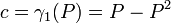
/* --------------- inverse function of multiplier map : explicit function : c=gamma_p(P) where P = w/(2^period) ---------------- */
gamma1(P):=P-P^2;
gamma2(P):=P - 1;
gamma3a(P):=(-(sqrt(3)*%i)/2-1/2)*(((P-1)*sqrt(27*P^2-22*P+23))/(6*sqrt(3))-(27*P^2-36*P+25)/54)^(1/3)+
(((sqrt(3)*%i)/2-1/2)*(3*P+1))/(9*(((P-1)*sqrt(27*P^2-22*P+23))/(6*sqrt(3))-(27*P^2-36*P+25)/54)^(1/3))-2/3;
gamma3b(P):=((sqrt(3)*%i)/2-1/2)*(((P-1)*sqrt(27*P^2-22*P+23))/(6*sqrt(3))-(27*P^2-36*P+25)/54)^(1/3)+
((-(sqrt(3)*%i)/2-1/2)*(3*P+1))/(9*(((P- 1)*sqrt(27*P^2-22*P+23))/(6*sqrt(3))-(27*P^2-36*P+25)/54)^(1/3))-2/3;
gamma3c(P):=(((P-1)*sqrt(27*P^2-22*P+23))/(6*sqrt(3))-(27*P^2-36*P+25)/54)^(1/3)+(3*P+1)/(9*(((P-1)*sqrt(27*P^2-22*P+23))/(6*sqrt(3))-
(27*P^2-36*P+25) /54)^(1/3))-2/3;
/* ---------- boundary equation (implicit function) b_p(P,c)=0 ------------------------------------------------------------------ */
b4(P):=c^6 + 3*c^5 + (P+3)* c^4 + (P+3)* c^3 - (P+2)*(P-1)*c^2 - (P-1)^3;
/* ------ period 5 ------------- */
b5(P):=c^15 +
8*c^14 +
28*c^13 +
(P + 60)*c^12 +
(7*P + 94)*c^11 +
(3*(P)^2 + 20*P + 116)*c^10 +
(11*P^2 + 33*P + 114)*c^9 +
(6*P^2 + 40*P + 94)*c^8 +
(2*P^3 - 20*P^2 + 37*P + 69)*c^7 +
(3*P - 11)*(3*P^2 - 3*P - 4)*c^6 +
(P - 1)*(3*P^3 + 20*P^2 - 33*P - 26)*c^5 +
(3*P^2 + 27*P + 14)*((P - 1)^2)*c^4 -
(6*P + 5)*((P - 1)^3 )*c^3 +
(P + 2)*((P - 1)^4)*c^2 -
c*(P - 1)^5 +
(P - 1)^6 ;
/*-----period 6 ----------------------- */
b6(P):=
c^27+
13*c^26+
78*c^25+
(293 - P)*c^24+
(792 - 10*P)*c^23+
(1672 - 41*P)*c^22+
(2892 - 84*P - 4*P^2)*c^21+
(4219 - 60*P - 30*P^2)*c^20+
(5313 + 155*P - 80*P^2)*c^19+
(5892 + 642*P - 57*P^2 + 4*P^3)*c^18+
(5843 + 1347*P + 195*P^2 + 22*P^3)*c^17+
(5258 + 2036*P + 734*P^2 + 22*P^3)*c^16+
(4346 + 2455*P + 1441*P^2 - 112*P^3 + 6*P^4)*c^15 +
(3310 + 2522*P + 1941*P^2 - 441*P^3 + 20*P^4)*c^14 +
(2331 + 2272*P + 1881*P^2 - 853*P^3 - 15*P^4)*c^13 +
(1525 + 1842*P + 1344*P^2 - 1157*P^3 - 124*P^4 - 6*P^5)*c^12 +
(927 + 1385*P + 570*P^2 - 1143*P^3 - 189*P^4 - 14*P^5)*c^11 +
(536 + 923*P - 126*P^2 - 774*P^3 - 186*P^4 + 11*P^5)*c^10 +
(298 + 834*P + 367*P^2 + 45*P^3 - 4*P^4 + 4*P^5)*(1-P)*c^9 +
(155 + 445*P - 148*P^2 - 109*P^3 + 103*P^4 + 2*P^5)*(1-P)*c^8 +
2*(38 + 142*P - 37*P^2 - 62*P^3 + 17*P^4)*(1-P)^2*c^7 +
(35 + 166*P + 18*P^2 - 75*P^3 - 4*P^4)*((1-P)^3)*c^6 +
(17 + 94*P + 62*P^2 + 2*P^3)*((1-P)^4)*c^5 +
(7 + 34*P + 8*P^2)*((1-P)^5)*c^4 +
(3 + 10*P + P^2)*((1-P)^6)*c^3 +
(1 + P)*((1-P)^7)*c^2 +
-c*((1-P)^8) + (1-P)^9;
/*-----------------------------------*/
/* point to point method of drawing */
t:0; /* angle in turns */
/* compute first point of curve, create list and save point to this list */
/* point of unit circle w:l(t); */
w:rectform(ev(l(t), numer)); /* "exponential form prevents allroots from working", code by Robert P. Munafo */
/* ---- period 1 -------------------*/
P:w/2;
c1:gamma1(P);
xx1:makelist (realpart(c1), i, 1, 1); /* save coordinates to draw it later */
yy1:makelist (imagpart(c1), i, 1, 1);
/* -----period 2 --------------*/
P:P/2;
c2:gamma2(P);
xx2:makelist (realpart(c2), i, 1, 1);
yy2:makelist (imagpart(c2), i, 1, 1);
/* period 3 components */
P:P/2;
c3:gamma3a(P);
xx3a:makelist (realpart(c3), i, 1, 1);
yy3a:makelist (imagpart(c3), i, 1, 1);
c3:gamma3b(w);
xx3b:makelist (realpart(c3), i, 1, 1);
yy3b:makelist (imagpart(c3), i, 1, 1);
c3:gamma3c(w);
xx3c:makelist (realpart(c3), i, 1, 1);
yy3c:makelist (imagpart(c3), i, 1, 1);
/* period 4 */
P:P/2;
per4:expand(b4(P)); /* compute equation for given w ( t) */
cc4:allroots(per4); /* compute 6 complex roots and save them to the list cc4 */
/* create new lists and save coordinates to draw it later */
xx4:makelist (realpart(rhs(cc4[1])), i, 1, 1);
yy4:makelist (imagpart(rhs(cc4[1])), i, 1, 1);
for j:2 thru 6 step 1 do
block
(
xx4:cons(realpart(rhs(cc4[j])),xx4),
yy4:cons(imagpart(rhs(cc4[j])),yy4)
);
/* period 5 */
P:P/2;
per5:expand(b5(P)); /* compute equation for given w ( t) */
cc5:allroots(per5); /* compute 15 complex roots and save them to the list cc5 */
/* create new lists and save coordinates to draw it later */
xx5:makelist (realpart(rhs(cc5[1])), i, 1, 1);
yy5:makelist (imagpart(rhs(cc5[1])), i, 1, 1);
for j:2 thru 15 step 1 do
block
(
xx5:cons(realpart(rhs(cc5[j])),xx5),
yy5:cons(imagpart(rhs(cc5[j])),yy5)
);
/* period 6 */
P:P/2;
per6:expand(b6(P)); /* compute equation for given w ( t) */
cc6:allroots(per6); /* compute 15 complex roots and save them to the list cc5 */
/* create new lists and save coordinates to draw it later */
xx6:makelist (realpart(rhs(cc6[1])), i, 1, 1);
yy6:makelist (imagpart(rhs(cc6[1])), i, 1, 1);
for j:2 thru 27 step 1 do
block
(
xx6:cons(realpart(rhs(cc6[j])),xx6),
yy6:cons(imagpart(rhs(cc6[j])),yy6)
);
/* ------------*/
for i:2 thru iMax step 1 do
block
( t:t+dt,
w:rectform(ev(l(t), numer)), /* "exponential form prevents allroots from working", code by Robert P. Munafo */
P:w/2,
c1:gamma1(P),
/* save values to draw it later */
xx1:cons(realpart(c1),xx1),
yy1:cons(imagpart(c1),yy1),
P:P/2,
c2:gamma2(P),
xx2:cons(realpart(c2),xx2),
yy2:cons(imagpart(c2),yy2),
P:P/2,
c3:gamma3a(P),
xx3a:cons(realpart(c3),xx3a),
yy3a:cons(imagpart(c3),yy3a),
c3:gamma3b(P),
xx3b:cons(realpart(c3),xx3b),
yy3b:cons(imagpart(c3),yy3b),
c3:gamma3c(P),
xx3c:cons(realpart(c3),xx3c),
yy3c:cons(imagpart(c3),yy3c),
/* period 4 */
P:P/2,
per4:expand(b4(P)),
cc4:allroots(per4),
for j:1 thru 6 step 1 do
block
(
xx4:cons(realpart(rhs(cc4[j])),xx4),
yy4:cons(imagpart(rhs(cc4[j])),yy4)
),
/* period 5 */
P:P/2,
per5:expand(b5(P)), /* compute equation for given w ( t) */
cc5:allroots(per5), /* compute 15 complex roots and save them to the list cc5 */
for j:1 thru 15 step 1 do
block
(
xx5:cons(realpart(rhs(cc5[j])),xx5),
yy5:cons(imagpart(rhs(cc5[j])),yy5)
),
/* period 6 */
P:P/2,
per6:expand(b6(P)), /* compute equation for given w ( t) */
cc6:allroots(per6), /* compute 27 complex roots and save them to the list cc6 */
for j:1 thru 27 step 1 do
block
(
xx6:cons(realpart(rhs(cc6[j])),xx6),
yy6:cons(imagpart(rhs(cc6[j])),yy6)
)
);
stop:elapsed_run_time ();
time:fix(stop-start);
load(draw);
draw2d(
user_preamble="set terminal svg size 1000,1000;set out 'mysvg2.svg';set size square;set key out vert;set key bot center",
pic_width = 1000,
pic_height = 1000,
yrange = [-1.5,1.5],
xrange = [-2,1],
title= concat("Boundaries of 53 hyperbolic components of Mandelbrot set made in ",string(time),"sec"),
xlabel = "c.re ",
ylabel = "c.im",
point_type = dot,
point_size = 5,
points_joined =true,
key = "one period 1 component = {c:c=(2*w-w*w)/4} ",
color = red,
points(xx1,yy1),
key = "one period 2 component = {c:c=(w/4 -1)} ",
color = green,
points(xx2,yy2),
key = "",
color = red,
points_joined =false, /* there are 3 curves so we can't join points */
points(xx3a,yy3a),
points(xx3b,yy3b),
key = "three period 3 components (blue)",
points(xx3c,yy3c),
key = "six period 4 components (magenta)",
color = red,
points(xx4,yy4),
key = "fifteen period 5 components (black)",
color = red,
points(xx5,yy5),
key = "27 period 6 components (black)",
colour = red,
points(xx6,yy6)
);
References
- ↑ Mario Rodriguez proposition in discussion about discrete dynamical system on the Maxima mailing list
- ↑ Multipliers of periodic orbits of quadratic polynomials and the parameter plane by Genadi Levin
- ↑ Algebraic solution of Mandelbrot orbital boundaries by Donald D. Cross
- ↑ A. Brown, Equations for Periodic Solutions of a Logistic Difference Equation, J. Austral. Math. Soc (Series B) 23, 78–94 (1981).
- ↑ John Stephenson : "Formulae for cycles in the Mandelbrot set", Physica A 177, 416-420 (1991); "Formulae for cycles in the Mandelbrot set II", Physica A 190, 104-116 (1992); "Formulae for cycles in the Mandelbrot set III", Physica A 190, 117-129 (1992)
- ↑ Wolf Jung : "Some Explicit Formulas for the Iteration of Rational Functions" , unpublished manuscript of August 1997 containing Maple code
- ↑ Thayer Watkins : The Structure of the Mandelbrot Set
- ↑ Enumeration of Features by Robert P. Munafo
- ↑ M. Lutzky: Counting hyperbolic components of the Mandelbrot set. Physics Letters A Volume 177, Issues 4-5, 21 June 1993, Pages 338-340
- ↑ Brown Method by Robert P. Munafo
- ↑ A Parameterization of the Period 3 Hyperbolic Components of the Mandelbrot Set Dante Giarrusso; Yuval Fisher Proceedings of the American Mathematical Society, Vol. 123, No. 12. (Dec., 1995), pp. 3731-3737
- ↑ Exact Coordinates by Robert P. Munafo
Acknowledgements
This program is not only my work but was done with help of many great people (see references). Warm thanks (:-))
Licensing
| This file is licensed under the Creative Commons Attribution-Share Alike 3.0 Unported license. | ||
|
|
|
This vector image was created with gnuplot. |
![]() ✓ The source code of this SVG is valid.
✓ The source code of this SVG is valid.
File usage
Metadata
Learn more
Wikipedia for Schools is one of SOS Children's Villages' many educational projects. SOS Childrens Villages helps those who have nothing and no one, giving them back the famly they have lost and bringing them the very best opportunities for a happy, healthy future. You can help by sponsoring a child.